

Bayesian Thinking for Data Scientists: Priors, Posteriors, and Intuition?
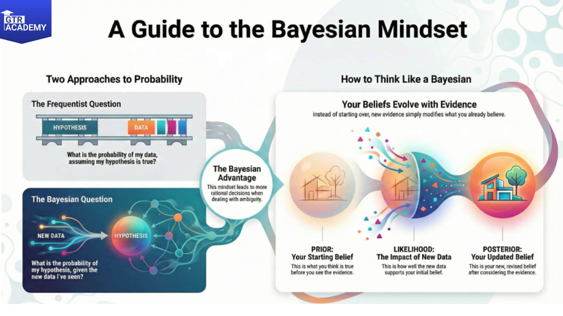
Frequentist stats basically consider something like “What is the probability of the Data Scientists if the hypothesis is true?” while Bayesian mindset is more like “What is the probability of the hypothesis if the data is given?”.
This change of mindset results in more natural uncertainty estimates and more rational decisions under ambiguity.
Connect With Us: WhatsApp
Bayesian basics without equations
In simple words Bayes’ theorem is:
Posterior = (Likelihood Prior) / Evidence
- Prior: What you think before the experiment (weak/strong prior).
- Likelihood: How well the data agrees with the hypothesis.
- Posterior: Updated belief after getting the data.
- Evidence: Normalizing (adjusting) constant (usually numerically computed).
- Intuition: New evidence modifies your prior beliefs instead of you having to start from scratch every time.
Frequentist vs Bayesian: churn probability example
Scenario: 10 customers tried a new feature; 3 churned. What’s the churn rate?
- Frequentist: Point estimate = 30% (3/10). 95% CI: 6.7–65%.
Bayesian:
-
- Start with weak prior (Beta (1,1) = uniform 0–100%).
- Update to posterior Beta (4,8) → mean 33%, 95% credible interval 11–60%.
- Strong prior (Beta (2,8) from past features) → posterior mean 29%.
Bayesian naturally incorporates domain knowledge via priors and gives interpretable intervals.
Why Bayesian thinking helps data scientists
Practical benefits:
- Uncertainty that’s intuitive: “90% credible interval for churn: 15–45%” vs opaque p‑values.
- Sequential updating: Easy to incorporate new data over time.
- Decision‑oriented: Directly answers “Should we ship given current evidence?”
- Hierarchical models: Pool information across groups/segments.
Tools and when to use them
Start simple:
- Pym, Stan: Full Bayesian modeling.
- scikit‑learn Bayesian Ridge: Drop‑in replacement for linear regression.
- Conjugate priors: Closed‑form updates for common cases (Beta‑Binomial, Normal‑Normal).
Use Bayesian when:
- Small data + strong domain priors.
- Need to update models over time.
- Decisions depend on full uncertainty distribution.
Try this: Fit a Bayesian churn model to a small dataset using a Beta prior. Compare posterior mean/interval to frequentist CI. Notice how priors pull estimates toward domain knowledge.